Ordinary Least Squares (OLS)
Ordinary Least Squares (OLS) 선형 회귀분석을 수행합니다.
Syntax
OrdinaryLeastSquares (SimpleFeatureCollection inputFeatures, String dependentVariable, String explanatoryVariables) : SimpleFeatureCollection, SpatialOLSResult
Input Parameters
Identifier |
Description |
Type |
Default |
Required |
inputFeatures |
종속변수와 독립변수를 포함하고 있는 입력 레이어입니다. |
SimpleFeatureCollection |
✓ |
|
dependentVariable |
종속변수값을 가진 숫자 필드입니다. |
String |
✓ |
|
explanatoryVariables |
회귀 분석에 사용할 쉼표로 구분된 설명 변수 숫자 필드의 목록입니다. |
String |
✓ |
Process Outputs
Identifier |
Description |
Type |
Default |
Required |
olsFeatures |
종속 변수 추정치와 잔차를 포함한 출력 레이어입니다. |
SimpleFeatureCollection |
||
report |
OLS 분석 결과입니다. |
SpatialOLSResult |
✓ |
Constraints
olsFeatures 레이어는 inputFeatures의 모든 필드를 포함해서 Estimated, Residual, StdResid, StdResid2 필드가 추가된다.
report 결과는 XML로 반환된다.
Examples
a1_2000 필드를 종속변수로, a2_2000, a3_2000, a4_2000 필드를 설명변수로 분석한 결과는 다음의 XML 포맷으로 반환됩니다.
<?xml version="1.0" encoding="UTF-8"?>
<OrdinaryLeastSquares>
  <ModelName>Ordinary Least Squares(OLS) Regression</ModelName>
  <Dataset>seoul_series</Dataset>
  <DependentVariable>a1_2000</DependentVariable>
  <NumberOfObservations>25</NumberOfObservations>
  <NumberOfVariables>4</NumberOfVariables>
  <DegreesOfFreedom>21</DegreesOfFreedom>
  <MeanDependentVar>18229.716524000003</MeanDependentVar>
  <SdDependentVar>5222.973372203831</SdDependentVar>
  <RSquared>0.2524024367985146</RSquared>
  <AdjustedRSquared>0.14560278491258805</AdjustedRSquared>
  <SumSquaredResidual>4.8945722348412424E8</SumSquaredResidual>
  <SigmaSquare>2.3307486832577344E7</SigmaSquare>
  <SeOfRegression>4827.782807104866</SeOfRegression>
  <SigmaSquareML>1.957828893936497E7</SigmaSquareML>
  <SeOfRegressionML>4424.736030472888</SeOfRegressionML>
  <FStatistic>2.363326399800135</FStatistic>
  <PValue>0.10015684828181148</PValue>
  <LogLikelihood>-245.3476108684226</LogLikelihood>
  <AIC>498.6952217368452</AIC>
  <AICc>503.8531164736873</AICc>
  <SchwarzCriterion>503.57072503631804</SchwarzCriterion>
  <Summary>
    <Variable>
      <Variable>CONSTANT</Variable>
      <Coefficient>-89839.01661165891</Coefficient>
      <StandardError>45251.64301979817</StandardError>
      <TStatistic>-1.9853205456507557</TStatistic>
      <Probability>0.060320415845298396</Probability>
    </Variable>
    <Variable>
      <Variable>a2_2000</Variable>
      <Coefficient>1015.5016202521613</Coefficient>
      <StandardError>459.27386712849943</StandardError>
      <TStatistic>2.2111025532572612</TStatistic>
      <Probability>0.03825397847242593</Probability>
    </Variable>
    <Variable>
      <Variable>a3_2000</Variable>
      <Coefficient>657.585445515956</Coefficient>
      <StandardError>687.1537990129104</StandardError>
      <TStatistic>0.9569698173255696</TStatistic>
      <Probability>0.3494719862156815</Probability>
    </Variable>
    <Variable>
      <Variable>a4_2000</Variable>
      <Coefficient>74.91087027691356</Coefficient>
      <StandardError>575.0254410828144</StandardError>
      <TStatistic>0.13027401037396014</TStatistic>
      <Probability>0.8975891001920921</Probability>
    </Variable>
  </Summary>
  <VarianceInflationFactor>
    <VIF>
      <Variable>a2_2000</Variable>
      <Value>1.0512492909076563</Value>
    </VIF>
    <VIF>
      <Variable>a3_2000</Variable>
      <Value>1.219785000060916</Value>
    </VIF>
    <VIF>
      <Variable>a4_2000</Variable>
      <Value>1.178277144719415</Value>
    </VIF>
  </VarianceInflationFactor>
  <Multicollinearity>124.00930330161376</Multicollinearity>
  <NormOfErrors>
    <Diagnostics>
      <Category>Test on Normality of Errors</Category>
      <Name>Jarque-Bera</Name>
      <DeegreesOfFreedom>2.0</DeegreesOfFreedom>
      <Value>0.7273519517018467</Value>
      <Probability>0.6951163927538146</Probability>
    </Diagnostics>
  </NormOfErrors>
  <HrcDiagnostics>
    <Diagnostics>
      <Category>Diagnostics for Heteroskedasticity Random Coefficients</Category>
      <Name>Breusch-Pagan</Name>
      <DeegreesOfFreedom>3.0</DeegreesOfFreedom>
      <Value>5.083212261808894</Value>
      <Probability>0.16580435989410658</Probability>
    </Diagnostics>
    <Diagnostics>
      <Category>Diagnostics for Heteroskedasticity Random Coefficients</Category>
      <Name>Koenker-Bassett</Name>
      <DeegreesOfFreedom>3.0</DeegreesOfFreedom>
      <Value>6.588607922676707</Value>
      <Probability>0.08623276842110539</Probability>
    </Diagnostics>
  </HrcDiagnostics>
</OrdinaryLeastSquares>
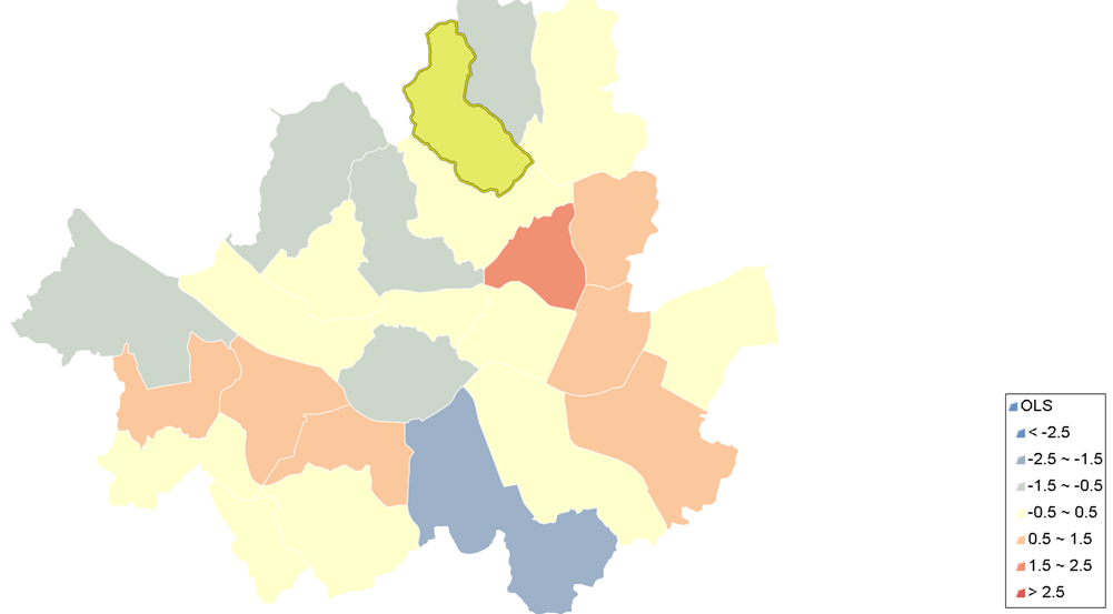
잔차를 이용한 시각화 결과입니다.